Extracting data from VCF files
This post gives an introduction to functions for extracting data from Variant Call Format (VCF) files and loading into NumPy arrays, pandas data frames, HDF5 files or Zarr arrays for ease of analysis. These functions are available in scikit-allel version 1.1 or later. Any feedback or bug reports welcome.
Update 2018-10-12: This post has been updated to use scikit-allel 1.1.10 and zarr 2.2, and adds examples of how to store data grouped by chromosome.
Introduction
Variant Call Format (VCF)
VCF is a widely-used file format for genetic variation data. Here is an example of a small VCF file, based on the example given in the VCF specification:
with open('example.vcf', mode='r') as vcf:
    print(vcf.read())
##fileformat=VCFv4.3
##reference=file:///seq/references/1000GenomesPilot-NCBI36.fasta
##contig=<ID=20,length=62435964,assembly=B36,md5=f126cdf8a6e0c7f379d618ff66beb2da,species="Homo sapiens",taxonomy=x>
##INFO=<ID=DP,Number=1,Type=Integer,Description="Total Depth">
##INFO=<ID=AF,Number=A,Type=Float,Description="Allele Frequency">
##INFO=<ID=DB,Number=0,Type=Flag,Description="dbSNP membership, build 129">
##FILTER=<ID=q10,Description="Quality below 10">
##FILTER=<ID=s50,Description="Less than 50% of samples have data">
##FORMAT=<ID=GT,Number=1,Type=String,Description="Genotype">
##FORMAT=<ID=DP,Number=1,Type=Integer,Description="Read Depth">
#CHROM POS ID REF ALT QUAL FILTER INFO FORMAT NA00001 NA00002 NA00003
20 14370 rs6054257 G A 29 PASS DP=14;AF=0.5;DB GT:DP 0/0:1 0/1:8 1/1:5
20 17330 . T A 3 q10 DP=11;AF=0.017 GT:DP 0/0:3 0/1:5 0/0:41
20 1110696 rs6040355 A G,T 67 PASS DP=10;AF=0.333,0.667;DB GT:DP 0/2:6 1/2:0 2/2:4
20 1230237 . T . 47 PASS DP=13 GT:DP 0/0:7 0/0:4 ./.:.
20 1234567 microsat1 GTC G,GTCT 50 PASS DP=9 GT:DP 0/1:4 0/2:2 1/1:3
A VCF file begins with a number of meta-information lines, which start with two hash (‘##’) characters. Then there is a single header line beginning with a single hash (‘#’) character. After the header line there are data lines, with each data line describing a genetic variant at a particular position relative to the reference genome of whichever species you are studying. Each data line is divided into fields separated by tab characters. There are 9 fixed fields, labelled “CHROM”, “POS”, “ID”, “REF”, “ALT”, “QUAL”, “FILTER”, “INFO” and “FORMAT”. Following these are fields containing data about samples, which usually contain a genotype call for each sample plus some associated data.
For example, the first data line in the file above describes a variant on chromosome 20 at position 14370 relative to the B36 assembly of the human genome. The reference allele is ‘G’ and the alternate allele is ‘A’, so this is a single nucleotide polymorphism (SNP). In this file there are three fields with data about samples labelled ‘NA00001’, ‘NA00002’ and ‘NA00003’. The genotype call in the first sample is ‘0/0’, meaning that individual ‘NA0001’ is homozygous for the reference allele at this position. The genotype call for the second sample is ‘0/1’ (you may need to scroll across to see this), which means that individual ‘NA00002’ is heterozygous for the reference and alternate alleles at this position.
NumPy, pandas, HDF5, Zarr, …
There are a number of software tools that can read VCF files and perform various analyses. However, if your dataset is large and/or you need to do some bespoke analysis, then it can be faster and more convenient to first extract the necessary data from the VCF file and load into a more efficient storage container.
For analysis and plotting of numerical data in Python, it is very convenient to load data into NumPy arrays. A NumPy array is an in-memory data structure that provides support for fast arithmetic and data manipulation. For analysing tables of data, pandas DataFrames provide useful features such as querying, aggregation and joins. When data are too large to fit into main memory, HDF5 files and Zarr arrays can provide fast on-disk storage and retrieval of numerical arrays.
scikit-allel is a Python package intended to enable exploratory analysis of large-scale genetic variation data. Version 1.1.0 of scikit-allel adds some new functions for extracting data from VCF files and loading the data into NumPy arrays, pandas DataFrames or HDF5 files. Once you have extracted these data, there are many analyses that can be run interactively on a commodity laptop or desktop computer, even with large-scale datasets from population resequencing studies. To give a flavour of what analyses can be done, there are a few previous articles on my blog, touching on topics including variant and sample QC, allele frequency differentiation, population structure, and genetic crosses.
Until now, getting data out of VCF files and into NumPy etc. has been a bit of a pain point. Hopefully the new scikit-allel functions will make this a bit less of a hurdle. Let’s take a look at the new functions…
read_vcf()
Let’s start with the scikit-allel function read_vcf(). First, some imports:
# import scikit-allel
import allel
# check which version is installed
print(allel.__version__)
1.1.10
Read the example VCF file shown above, using default parameters:
callset = allel.read_vcf('example.vcf')The callset object returned by read_vcf() is a Python dictionary (dict). It contains several NumPy arrays, each of which can be accessed via a key. Here are the available keys:
sorted(callset.keys())['calldata/GT',
'samples',
'variants/ALT',
'variants/CHROM',
'variants/FILTER_PASS',
'variants/ID',
'variants/POS',
'variants/QUAL',
'variants/REF']
The ‘samples’ array contains sample identifiers extracted from the header line in the VCF file.
callset['samples']array(['NA00001', 'NA00002', 'NA00003'], dtype=object)
All arrays with keys beginning ‘variants/’ come from the fixed fields in the VCF file. For example, here is the data from the ‘CHROM’ field:
callset['variants/CHROM']array(['20', '20', '20', '20', '20'], dtype=object)
Here is the data from the ‘POS’ field:
callset['variants/POS']array([ 14370, 17330, 1110696, 1230237, 1234567], dtype=int32)
Here is the data from the ‘QUAL’ field:
callset['variants/QUAL']array([ 29., 3., 67., 47., 50.], dtype=float32)
All arrays with keys beginning ‘calldata/’ come from the sample fields in the VCF file. For example, here are the actual genotype calls from the ‘GT’ field:
callset['calldata/GT']array([[[ 0, 0],
[ 0, 1],
[ 1, 1]],
[[ 0, 0],
[ 0, 1],
[ 0, 0]],
[[ 0, 2],
[ 1, 2],
[ 2, 2]],
[[ 0, 0],
[ 0, 0],
[-1, -1]],
[[ 0, 1],
[ 0, 2],
[ 1, 1]]], dtype=int8)
Note the -1 values for one of the genotype calls. By default scikit-allel uses -1 to indicate a missing value for any array with a signed integer data type (although you can change this if you want).
Aside: genotype arrays
Because working with genotype calls is a very common task, scikit-allel has a GenotypeArray class which adds some convenient functionality to an array of genotype calls. To use this class, pass the raw NumPy array into the GenotypeArray class constructor, e.g.:
gt = allel.GenotypeArray(callset['calldata/GT'])
gt| 0 | 1 | 2 | |
|---|---|---|---|
| 0 | 0/0 | 0/1 | 1/1 |
| 1 | 0/0 | 0/1 | 0/0 |
| 2 | 0/2 | 1/2 | 2/2 |
| 3 | 0/0 | 0/0 | ./. |
| 4 | 0/1 | 0/2 | 1/1 |
One of the things that the GenotypeArray class does is provide a slightly more visually-appealing representation when used in a Jupyter notebook, as can be seen above. There are also methods for making various computations over the genotype calls. For example, the is_het() method locates all heterozygous genotype calls:
gt.is_het()array([[False, True, False],
[False, True, False],
[ True, True, False],
[False, False, False],
[ True, True, False]], dtype=bool)
To give another example, the count_het() method will count heterozygous calls, summing over variants (axis=0) or samples (axis=1) if requested. E.g., to count the number of het calls per variant:
gt.count_het(axis=1)array([1, 1, 2, 0, 2])
One more example, here is how to perform an allele count, i.e., count the number times each allele (0=reference, 1=first alternate, 2=second alternate, etc.) is observed for each variant:
ac = gt.count_alleles()
ac| 0 | 1 | 2 | |
|---|---|---|---|
| 0 | 3 | 3 | 0 |
| 1 | 5 | 1 | 0 |
| 2 | 1 | 1 | 4 |
| 3 | 4 | 0 | 0 |
| 4 | 2 | 3 | 1 |
Fields
VCF files can often contain many fields of data, and you may only need to extract some of them to perform a particular analysis. You can select which fields to extract by passing a list of strings as the fields parameter. For example, let’s extract the ‘DP’ field from within the ‘INFO’ field, and let’s also extract the ‘DP’ field from the genotype call data:
callset = allel.read_vcf('example.vcf', fields=['variants/DP', 'calldata/DP'])
sorted(callset.keys())
['calldata/DP', 'variants/DP']
Here is the data that we just extracted:
callset['variants/DP']array([14, 11, 10, 13, 9], dtype=int32)
callset['calldata/DP']array([[ 1, 8, 5],
[ 3, 5, 41],
[ 6, 0, 4],
[ 7, 4, -1],
[ 4, 2, 3]], dtype=int16)
I chose these two fields to illustrate the point that sometimes the same field name (e.g., ‘DP’) can be used both within the INFO field of a VCF and also within the genotype call data. When selecting fields, to make sure there is no ambiguity, you can include a prefix which is either ‘variants/’ or ‘calldata/’. For example, if you provide ‘variants/DP’, then the read_vcf() function will look for an INFO field named ‘DP’. If you provide ‘calldata/DP’ then read_vcf() will look for a FORMAT field named ‘DP’ within the call data.
If you are feeling lazy, you can drop the ‘variants/’ and ‘calldata/’ prefixes, in which case read_vcf() will assume you mean ‘variants/’ if there is any ambiguity. E.g.:
callset = allel.read_vcf('example.vcf', fields=['DP', 'GT'])
sorted(callset.keys())
['calldata/GT', 'variants/DP']
If you want to extract absolutely everything from a VCF file, then you can provide a special value '*' as the fields parameter:
callset = allel.read_vcf('example.vcf', fields='*')
sorted(callset.keys())
['calldata/DP',
'calldata/GT',
'samples',
'variants/AF',
'variants/ALT',
'variants/CHROM',
'variants/DB',
'variants/DP',
'variants/FILTER_PASS',
'variants/FILTER_q10',
'variants/FILTER_s50',
'variants/ID',
'variants/POS',
'variants/QUAL',
'variants/REF',
'variants/is_snp',
'variants/numalt',
'variants/svlen']
You can also provide the special value 'variants/*' to request all variants fields (including all INFO), and the special value 'calldata/*' to request all call data fields.
If you don’t specify the fields parameter, scikit-allel will default to extracting data from the fixed variants fields (but no INFO) and the GT genotype field if present (but no other call data).
Types
NumPy arrays can have various data types, including signed integers (‘int8’, ‘int16’, ‘int32’, ‘int64’), unsigned integers (‘uint8’, ‘uint16’, ‘uint32’, ‘uint64’), floating point numbers (‘float32’, ‘float64’), variable length strings (‘object’) and fixed length strings (e.g., ‘S4’ for a 4-character ASCII string). scikit-allel will try to choose a sensible default data type for the fields you want to extract, based on the meta-information in the VCF file, but you can override these via the types parameter.
For example, by default the ‘DP’ INFO field is loaded into a 32-bit integer array:
callset = allel.read_vcf('example.vcf', fields=['DP'])
callset['variants/DP']
array([14, 11, 10, 13, 9], dtype=int32)
If you know the maximum value this field is going to contain, to save some memory you could choose a 16-bit integer array instead:
callset = allel.read_vcf('example.vcf', fields=['DP'], types={'DP': 'int16'})
callset['variants/DP']
array([14, 11, 10, 13, 9], dtype=int16)
You can also choose a floating-point data type, even for fields that are declared as type ‘Integer’ in the VCF meta-information, and vice versa. E.g.:
callset = allel.read_vcf('example.vcf', fields=['DP'], types={'DP': 'float32'})
callset['variants/DP']
array([ 14., 11., 10., 13., 9.], dtype=float32)
For fields containing textual data, there are two choices for data type. By default, scikit-allel will use an ‘object’ data type, which means that values are stored as an array of Python strings. E.g.:
callset = allel.read_vcf('example.vcf')
callset['variants/REF']
array(['G', 'T', 'A', 'T', 'GTC'], dtype=object)
The advantage of using ‘object’ dtype is that strings can be of any length. Alternatively, you can use a fixed-length string dtype, e.g.:
callset = allel.read_vcf('example.vcf', types={'REF': 'S3'})
callset['variants/REF']
array([b'G', b'T', b'A', b'T', b'GTC'],
dtype='|S3')
Note that fixed-length string dtypes will cause any string values longer than the requested number of characters to be truncated. I.e., there can be some data loss. E.g., if using a single-character string for the ‘REF’ field, the correct value of ‘GTC’ for the final variant will get truncated to ‘G’:
callset = allel.read_vcf('example.vcf', types={'REF': 'S1'})
callset['variants/REF']
array([b'G', b'T', b'A', b'T', b'G'],
dtype='|S1')
Numbers
Some fields like ‘ALT’, ‘AC’ and ‘AF’ can have a variable number of values. I.e., each variant may have a different number of data values for these fields. One trade-off you have to make when loading data into NumPy arrays is that you cannot have arrays with a variable number of items per row. Rather, you have to fix the maximum number of possible items. While you lose some flexibility, you gain speed of access.
For fields like ‘ALT’, scikit-allel will choose a default number of expected values, which is set at 3. E.g., here is what you get by default:
callset = allel.read_vcf('example.vcf')
callset['variants/ALT']
array([['A', '', ''],
['A', '', ''],
['G', 'T', ''],
['', '', ''],
['G', 'GTCT', '']], dtype=object)
In this case, 3 is more that we need, because no variant has more than 2 ALT values. However, some VCF files (especially those including INDELs) may have more than 3 ALT values.
If you need to increase or decrease the expected number of values for any field, you can do this via the numbers parameter. E.g., increase the number of ALT values to 5:
callset = allel.read_vcf('example.vcf', numbers={'ALT': 5})
callset['variants/ALT']
array([['A', '', '', '', ''],
['A', '', '', '', ''],
['G', 'T', '', '', ''],
['', '', '', '', ''],
['G', 'GTCT', '', '', '']], dtype=object)
Some care is needed here, because if you choose a value that is lower than the maximum number of values in the VCF file, then any extra values will not get extracted. E.g., the following would be fine if all variants were biallelic, but would lose information for any multi-allelic variants:
callset = allel.read_vcf('example.vcf', numbers={'ALT': 1})
callset['variants/ALT']
array(['A', 'A', 'G', '', 'G'], dtype=object)
Number of alternate alleles
Often there will be several fields within a VCF that all have a number of values that depends on the number of alternate alleles (declared with number ‘A’ or ‘R’ in the VCF meta-information). You can set the expected number of values simultaneously for all such fields via the alt_number parameter:
callset = allel.read_vcf('example.vcf', fields=['ALT', 'AF'], alt_number=2)callset['variants/ALT']array([['A', ''],
['A', ''],
['G', 'T'],
['', ''],
['G', 'GTCT']], dtype=object)
callset['variants/AF']array([[ 0.5 , nan],
[ 0.017, nan],
[ 0.333, 0.667],
[ nan, nan],
[ nan, nan]], dtype=float32)
Genotype ploidy
By default, scikit-allel assumes you are working with a diploid organism, and so expects to parse out 2 alleles for each genotype call. If you are working with an organism with some other ploidy, you can change the expected number of alleles via the numbers parameter.
For example, here is an example VCF with tetraploid genotype calls:
with open('example_polyploid.vcf', mode='r') as f:
    print(f.read())
##fileformat=VCFv4.3
##FORMAT=<ID=GT,Number=1,Type=String,Description="Genotype">
#CHROM POS ID REF ALT QUAL FILTER INFO FORMAT sample1 sample2 sample3
20 14370 . G A . . . GT 0/0/0/0 0/0/0/1 0/0/1/1
20 17330 . T A,C,G . . . GT 1/1/2/2 0/1/2/3 3/3/3/3
Here is how to indicate the ploidy:
callset = allel.read_vcf('example_polyploid.vcf', numbers={'GT': 4})
callset['calldata/GT']
array([[[0, 0, 0, 0],
[0, 0, 0, 1],
[0, 0, 1, 1]],
[[1, 1, 2, 2],
[0, 1, 2, 3],
[3, 3, 3, 3]]], dtype=int8)
As shown earlier for diploid calls, the GenotypeArray class can provide some extra functionality over a plain NumPy array, e.g.:
gt = allel.GenotypeArray(callset['calldata/GT'])
gt| 0 | 1 | 2 | |
|---|---|---|---|
| 0 | 0/0/0/0 | 0/0/0/1 | 0/0/1/1 |
| 1 | 1/1/2/2 | 0/1/2/3 | 3/3/3/3 |
gt.is_het()array([[False, True, True],
[ True, True, False]], dtype=bool)
ac = gt.count_alleles()
ac| 0 | 1 | 2 | 3 | |
|---|---|---|---|---|
| 0 | 9 | 3 | 0 | 0 |
| 1 | 1 | 3 | 3 | 5 |
Region
You can extract data for only a specific chromosome or genome region via the region parameter. The value of the parameter should be a region string of the format ‘{chromosome}:{begin}-{end}’, just like you would give to tabix or samtools. E.g.:
callset = allel.read_vcf('example.vcf', region='20:1000000-1231000')
callset['variants/POS']
array([1110696, 1230237], dtype=int32)
By default, scikit-allel will try to use tabix to extract the data from the requested region. If tabix is not available on your system or the VCF file has not been tabix indexed, scikit-allel will fall back to scanning through the VCF file from the beginning, which may be slow. If you have tabix installed but it is in a non-standard location, you can specify the path to the tabix executable via the tabix parameter.
Note that if you are using tabix, then tabix needs to be at least version 0.2.5. Some older versions of tabix do not support the “-h” option to output the headers from the VCF, which scikit-allel needs to get the meta-information for parsing. If you get an error message like “RuntimeError: VCF file is missing mandatory header line (“#CHROM…”)” then check your tabix version and upgrade if necessary. If you have conda installed, a recent version tabix can be installed via the following command: conda install -c bioconda htslib.
Samples
You can extract data for only specific samples via the samples parameter. E.g., extract data for samples ‘NA00001’ and ‘NA00003’:
callset = allel.read_vcf('example.vcf', samples=['NA00001', 'NA00003'])
callset['samples']
array(['NA00001', 'NA00003'], dtype=object)
allel.GenotypeArray(callset['calldata/GT'])| 0 | 1 | |
|---|---|---|
| 0 | 0/0 | 1/1 |
| 1 | 0/0 | 0/0 |
| 2 | 0/2 | 2/2 |
| 3 | 0/0 | ./. |
| 4 | 0/1 | 1/1 |
Note that the genotype array now only has two columns, corresponding to the two samples requested.
vcf_to_npz()
NumPy arrays are stored in main memory (a.k.a., RAM), which means that as soon as you end your Python session or restart your Jupyter notebook kernel, any data stored in a NumPy array will be lost.
If your VCF file is not too big, you can extract data from the file into NumPy arrays then save those arrays to disk via the vcf_to_npz() function. This function has most of the same parameters as the read_vcf() function, except that you also specify an output path, which is the name of the file you want to save the extracted data to. For example:
allel.vcf_to_npz('example.vcf', 'example.npz', fields='*', overwrite=True)This extraction only needs to be done once, then you can load the data any time directly into NumPy arrays via the NumPy load() function, e.g.:
import numpy as np
callset = np.load('example.npz')
callset
<numpy.lib.npyio.NpzFile at 0x7f829b07d6d8>
sorted(callset.keys())['calldata/DP',
'calldata/GT',
'samples',
'variants/AF',
'variants/ALT',
'variants/CHROM',
'variants/DB',
'variants/DP',
'variants/FILTER_PASS',
'variants/FILTER_q10',
'variants/FILTER_s50',
'variants/ID',
'variants/POS',
'variants/QUAL',
'variants/REF',
'variants/is_snp',
'variants/numalt',
'variants/svlen']
callset['variants/POS']array([ 14370, 17330, 1110696, 1230237, 1234567], dtype=int32)
callset['calldata/GT']array([[[ 0, 0],
[ 0, 1],
[ 1, 1]],
[[ 0, 0],
[ 0, 1],
[ 0, 0]],
[[ 0, 2],
[ 1, 2],
[ 2, 2]],
[[ 0, 0],
[ 0, 0],
[-1, -1]],
[[ 0, 1],
[ 0, 2],
[ 1, 1]]], dtype=int8)
Note that although the data have been saved to disk, all of the data must be loaded into main memory first during the extraction process, so this function is not suitable if you have a dataset that is too large to fit into main memory.
vcf_to_hdf5()
For large datasets, the vcf_to_hdf5() function is available. This function again takes similar parameters to read_vcf(), but will store extracted data into an HDF5 file stored on disk. The extraction process works through the VCF file in chunks, and so the entire dataset is never loaded entirely into main memory. A bit further below I give worked examples with a large dataset, but for now here is a simple example:
allel.vcf_to_hdf5('example.vcf', 'example.h5', fields='*', overwrite=True)The saved data can be accessed via the h5py library, e.g.:
import h5py
callset = h5py.File('example.h5', mode='r')
callset
<HDF5 file "example.h5" (mode r)>
The one difference to be aware of here is that accessing data via a key like ‘variants/POS’ does not return a NumPy array, instead you get an HDF5 dataset object.
chrom = callset['variants/CHROM']
chrom
<HDF5 dataset "CHROM": shape (5,), type "|O">
pos = callset['variants/POS']
pos
<HDF5 dataset "POS": shape (5,), type "<i4">
gt = callset['calldata/GT']
gt
<HDF5 dataset "GT": shape (5, 3, 2), type "|i1">
This dataset object is useful because you can then load all or only part of the underlying data into main memory via slicing. E.g.:
# load second to fourth items into NumPy array
chrom[1:3]
array(['20', '20'], dtype=object)
# load second to fourth items into NumPy array
pos[1:3]
array([ 17330, 1110696], dtype=int32)
# load all items into NumPy array
chrom[:]
array(['20', '20', '20', '20', '20'], dtype=object)
# load all items into NumPy array
pos[:]
array([ 14370, 17330, 1110696, 1230237, 1234567], dtype=int32)
This is particularly useful for the large data coming from the sample fields, e.g., the genotype calls. With these data you can use slicing to pull out particular rows or columns without having to load all data into memory. E.g.:
# load genotype calls into memory for second to fourth variants, all samples
allel.GenotypeArray(gt[1:3, :])| 0 | 1 | 2 | |
|---|---|---|---|
| 0 | 0/0 | 0/1 | 0/0 |
| 1 | 0/2 | 1/2 | 2/2 |
# load genotype calls into memory for all variants, first and second samples
allel.GenotypeArray(gt[:, 0:2])| 0 | 1 | |
|---|---|---|
| 0 | 0/0 | 0/1 |
| 1 | 0/0 | 0/1 |
| 2 | 0/2 | 1/2 |
| 3 | 0/0 | 0/0 |
| 4 | 0/1 | 0/2 |
# load all genotype calls into memory
allel.GenotypeArray(gt[:, :])| 0 | 1 | 2 | |
|---|---|---|---|
| 0 | 0/0 | 0/1 | 1/1 |
| 1 | 0/0 | 0/1 | 0/0 |
| 2 | 0/2 | 1/2 | 2/2 |
| 3 | 0/0 | 0/0 | ./. |
| 4 | 0/1 | 0/2 | 1/1 |
Storing strings
By default, scikit-allel will store data from string fields like CHROM, ID, REF and ALT in the HDF5 file as variable length strings. Unfortunately HDF5 uses a lot of space to store variable length strings, and so for larger datasets this can lead to very large HDF5 file sizes. You can disable this option by setting the vlen parameter to False, which will force all data from string fields to be stored as fixed length strings. For example:
allel.vcf_to_hdf5('example.vcf', 'example_novlen.h5', fields='*', overwrite=True, vlen=False)callset = h5py.File('example_novlen.h5', mode='r')callset['variants/ID']<HDF5 dataset "ID": shape (5,), type "|S9">
callset['variants/ID'][:]array([b'rs6054257', b'.', b'rs6040355', b'.', b'microsat1'],
dtype='|S9')
Note that an appropriate length to use for the fixed length string data type for each string field will be guessed from the longest string found for each field in the first chunk of the VCF. In some cases there may be longer strings found later in a VCF, in which case string values may get truncated. If you already know something about the longest value in a given field, you can specify types manually to avoid truncation, e.g.:
allel.vcf_to_hdf5('example.vcf', 'example_novlen_types.h5',
                  fields=['CHROM', 'ID'],
                  types={'CHROM': 'S2', 'ID': 'S10'},
                  overwrite=True, vlen=False)
callset = h5py.File('example_novlen_types.h5', mode='r')callset['variants/ID']<HDF5 dataset "ID": shape (5,), type "|S10">
vcf_to_zarr()
An alternative to HDF5 is a newer storage library called Zarr. Currently there is only a Python implementation of Zarr, whereas you can access HDF5 files using a variety of different programming languages, so if you need portability then HDF5 is a better option. However, if you know you’re only going to be using Python, then Zarr is a good option. In general it is a bit faster than HDF5, provides more storage and compression options, and also plays better with parellel computing libraries like Dask.
To install Zarr, from the command line, run: conda install -c conda-forge zarr
To extract data to Zarr, for example:
allel.vcf_to_zarr('example.vcf', 'example.zarr', fields='*', overwrite=True)Then, to access saved data:
import zarr
import numcodecs
print('zarr', zarr.__version__, 'numcodecs', numcodecs.__version__)
zarr 2.2.0 numcodecs 0.5.5
callset = zarr.open_group('example.zarr', mode='r')
callset
<zarr.hierarchy.Group '/' read-only>
Zarr group objects provide a tree() method which can be useful for exploring the hierarchy of groups and arrays, e.g.:
callset.tree(expand=True)- /
- calldata
- DP (5, 3) int16
- GT (5, 3, 2) int8
- samples (3,) object
- variants
- AF (5, 3) float32
- ALT (5, 3) object
- CHROM (5,) object
- DB (5,) bool
- DP (5,) int32
- FILTER_PASS (5,) bool
- FILTER_q10 (5,) bool
- FILTER_s50 (5,) bool
- ID (5,) object
- POS (5,) int32
- QUAL (5,) float32
- REF (5,) object
- is_snp (5,) bool
- numalt (5,) int32
- svlen (5, 3) int32
- calldata
As with h5py, arrays can be accessed via a path-like notation, e.g.:
chrom = callset['variants/CHROM']
chrom
<zarr.core.Array '/variants/CHROM' (5,) object read-only>
pos = callset['variants/POS']
pos
<zarr.core.Array '/variants/POS' (5,) int32 read-only>
gt = callset['calldata/GT']
gt
<zarr.core.Array '/calldata/GT' (5, 3, 2) int8 read-only>
Again as with h5py, data can be loaded into memory as numpy arrays via slice notation:
chrom[1:3]array(['20', '20'], dtype=object)
pos[1:3]array([ 17330, 1110696], dtype=int32)
chrom[:]array(['20', '20', '20', '20', '20'], dtype=object)
pos[:]array([ 14370, 17330, 1110696, 1230237, 1234567], dtype=int32)
allel.GenotypeArray(gt[1:3, :])| 0 | 1 | 2 | |
|---|---|---|---|
| 0 | 0/0 | 0/1 | 0/0 |
| 1 | 0/2 | 1/2 | 2/2 |
allel.GenotypeArray(gt[:, 0:2])| 0 | 1 | |
|---|---|---|
| 0 | 0/0 | 0/1 |
| 1 | 0/0 | 0/1 |
| 2 | 0/2 | 1/2 |
| 3 | 0/0 | 0/0 |
| 4 | 0/1 | 0/2 |
allel.GenotypeArray(gt[:])| 0 | 1 | 2 | |
|---|---|---|---|
| 0 | 0/0 | 0/1 | 1/1 |
| 1 | 0/0 | 0/1 | 0/0 |
| 2 | 0/2 | 1/2 | 2/2 |
| 3 | 0/0 | 0/0 | ./. |
| 4 | 0/1 | 0/2 | 1/1 |
vcf_to_dataframe()
For some analyses it can be useful to think of the data in a VCF file as a table or data frame, especially if you are only analysing data from the fixed fields and don’t need the genotype calls or any other call data. The vcf_to_dataframe() function extracts data from a VCF and loads into a pandas DataFrame. E.g.:
df = allel.vcf_to_dataframe('example.vcf')
df| CHROM | POS | ID | REF | ALT_1 | ALT_2 | ALT_3 | QUAL | FILTER_PASS | |
|---|---|---|---|---|---|---|---|---|---|
| 0 | 20 | 14370 | rs6054257 | G | A | 29.0 | True | ||
| 1 | 20 | 17330 | . | T | A | 3.0 | False | ||
| 2 | 20 | 1110696 | rs6040355 | A | G | T | 67.0 | True | |
| 3 | 20 | 1230237 | . | T | 47.0 | True | |||
| 4 | 20 | 1234567 | microsat1 | GTC | G | GTCT | 50.0 | True |
Note that the ‘ALT’ field has been broken into three separate columns, labelled ‘ALT_1’, ‘ALT_2’ and ‘ALT_3’. When loading data into a data frame, any field with multiple values will be broken into multiple columns in this way.
Let’s extract all fields, and also reduce number of values per field given that we know there are at most 2 alternate alleles in our example VCF file:
df = allel.vcf_to_dataframe('example.vcf', fields='*', alt_number=2)
df| CHROM | POS | ID | REF | ALT_1 | ALT_2 | QUAL | DP | AF_1 | AF_2 | DB | FILTER_PASS | FILTER_q10 | FILTER_s50 | numalt | svlen_1 | svlen_2 | is_snp | |
|---|---|---|---|---|---|---|---|---|---|---|---|---|---|---|---|---|---|---|
| 0 | 20 | 14370 | rs6054257 | G | A | 29.0 | 14 | 0.500 | NaN | True | True | False | False | 1 | 0 | 0 | True | |
| 1 | 20 | 17330 | . | T | A | 3.0 | 11 | 0.017 | NaN | False | False | True | False | 1 | 0 | 0 | True | |
| 2 | 20 | 1110696 | rs6040355 | A | G | T | 67.0 | 10 | 0.333 | 0.667 | True | True | False | False | 2 | 0 | 0 | True |
| 3 | 20 | 1230237 | . | T | 47.0 | 13 | NaN | NaN | False | True | False | False | 0 | 0 | 0 | False | ||
| 4 | 20 | 1234567 | microsat1 | GTC | G | GTCT | 50.0 | 9 | NaN | NaN | False | True | False | False | 2 | -2 | 1 | False |
In case you were wondering, the ‘numalt’, ‘svlen’ and ‘is_snp’ fields are computed by scikit-allel, they are not present in the original VCF.
Pandas DataFrames have many useful features. For example, you can query:
df.query('DP > 10 and QUAL > 20')| CHROM | POS | ID | REF | ALT_1 | ALT_2 | QUAL | DP | AF_1 | AF_2 | DB | FILTER_PASS | FILTER_q10 | FILTER_s50 | numalt | svlen_1 | svlen_2 | is_snp | |
|---|---|---|---|---|---|---|---|---|---|---|---|---|---|---|---|---|---|---|
| 0 | 20 | 14370 | rs6054257 | G | A | 29.0 | 14 | 0.5 | NaN | True | True | False | False | 1 | 0 | 0 | True | |
| 3 | 20 | 1230237 | . | T | 47.0 | 13 | NaN | NaN | False | True | False | False | 0 | 0 | 0 | False |
vcf_to_recarray()
If you prefer to work with NumPy structured arrays rather than pandas DataFrames, try the vcf_to_recarray() function, e.g.:
ra = allel.vcf_to_recarray('example.vcf')
ra
array([('20', 14370, 'rs6054257', 'G', 'A', '', '', 29., True),
('20', 17330, '.', 'T', 'A', '', '', 3., False),
('20', 1110696, 'rs6040355', 'A', 'G', 'T', '', 67., True),
('20', 1230237, '.', 'T', '', '', '', 47., True),
('20', 1234567, 'microsat1', 'GTC', 'G', 'GTCT', '', 50., True)],
dtype=(numpy.record, [('CHROM', 'O'), ('POS', '<i4'), ('ID', 'O'), ('REF', 'O'), ('ALT_1', 'O'), ('ALT_2', 'O'), ('ALT_3', 'O'), ('QUAL', '<f4'), ('FILTER_PASS', '?')]))
vcf_to_csv()
Finally, the vcf_to_csv() function is available if you need to dump data from a VCF file out to a generic CSV file (e.g., to load into a database). E.g.:
allel.vcf_to_csv('example.vcf', 'example.csv', fields=['CHROM', 'POS', 'DP'])with open('example.csv', mode='r') as f:
print(f.read())CHROM,POS,DP
20,14370,14
20,17330,11
20,1110696,10
20,1230237,13
20,1234567,9
This function uses the pandas to_csv() function under the hood to write the CSV, so you can control various output parameters (e.g., field separator) by passing through keyword arguments.
Worked example: human 1000 genomes phase 3
I’ve downloaded a VCF file with genotype data for Chromosome 22 from the 1000 genomes project phase 3 FTP site.
vcf_path = 'data/ALL.chr22.phase3_shapeit2_mvncall_integrated_v5a.20130502.genotypes.vcf.gz'Before we start processing, let’s see how big the file is (the ‘!’ is special Jupyter notebook syntax for running a command via the operating system shell):
!ls -lh {vcf_path}-rw-r--r-- 1 aliman aliman 205M Jun 20 2017 data/ALL.chr22.phase3_shapeit2_mvncall_integrated_v5a.20130502.genotypes.vcf.gz
…and how many lines:
!zcat {vcf_path} | wc -l1103800
So there are more than a million variants.
Preparation
When processing larger VCF files it’s useful to get some feedback on how fast things are going. Let’s import the sys module so we can log to standard output:
import sysUltimately I am going to extract all the data from this VCF file into a Zarr store. However, before I do that, I’m going to check how many alternate alleles I should expect. I’m going to do that by extracting just the ‘numalt’ field, which scikit-allel will compute from the number of values in the ‘ALT’ field:
callset = allel.read_vcf(vcf_path, fields=['numalt'], log=sys.stdout)[read_vcf] 65536 rows in 8.19s; chunk in 8.19s (8001 rows/s); 22�:18539397
[read_vcf] 131072 rows in 16.05s; chunk in 7.86s (8341 rows/s); 22�:21016127
[read_vcf] 196608 rows in 22.73s; chunk in 6.69s (9800 rows/s); 22�:23236362
[read_vcf] 262144 rows in 27.52s; chunk in 4.78s (13696 rows/s); 22�:25227844
[read_vcf] 327680 rows in 32.98s; chunk in 5.46s (12001 rows/s); 22�:27285434
[read_vcf] 393216 rows in 38.07s; chunk in 5.09s (12879 rows/s); 22�:29572822
[read_vcf] 458752 rows in 43.13s; chunk in 5.06s (12940 rows/s); 22�:31900536
[read_vcf] 524288 rows in 47.94s; chunk in 4.80s (13640 rows/s); 22�:34069864
[read_vcf] 589824 rows in 53.03s; chunk in 5.09s (12869 rows/s); 22�:36053392
[read_vcf] 655360 rows in 59.10s; chunk in 6.07s (10804 rows/s); 22�:38088395
[read_vcf] 720896 rows in 66.34s; chunk in 7.25s (9044 rows/s); 22�:40216200
[read_vcf] 786432 rows in 72.77s; chunk in 6.43s (10192 rows/s); 22�:42597446
[read_vcf] 851968 rows in 78.85s; chunk in 6.08s (10775 rows/s); 22�:44564263
[read_vcf] 917504 rows in 84.40s; chunk in 5.54s (11823 rows/s); 22�:46390672
[read_vcf] 983040 rows in 89.51s; chunk in 5.12s (12807 rows/s); 22�:48116697
[read_vcf] 1048576 rows in 95.96s; chunk in 6.45s (10162 rows/s); 22�:49713436
[read_vcf] 1103547 rows in 102.48s; chunk in 6.52s (8436 rows/s)
[read_vcf] all done (10768 rows/s)
Let’s see what the largest number of alternate alleles is:
numalt = callset['variants/numalt']
np.max(numalt)
8
Out of interest, how many variants are multi-allelic?
count_numalt = np.bincount(numalt)
count_numalt
array([ 0, 1097199, 6073, 224, 38, 9, 3,
0, 1])
n_multiallelic = np.sum(count_numalt[2:])
n_multiallelic
6348
So there are only a very small number of multi-allelic variants (6,348), the vast majority (1,097,199) have just one alternate allele.
Extract to Zarr
Now we know how many alternate alleles to expect, let’s go ahead and extract everything out into a Zarr on-disk store. Time for a cup of tea:
zarr_path = 'data/ALL.phase3_shapeit2_mvncall_integrated_v5a.20130502.genotypes.zarr'allel.vcf_to_zarr(vcf_path, zarr_path, group='22',
fields='*', alt_number=8, log=sys.stdout,
compressor=numcodecs.Blosc(cname='zstd', clevel=1, shuffle=False))[vcf_to_zarr] 65536 rows in 15.14s; chunk in 15.14s (4328 rows/s); 22�:18539397
[vcf_to_zarr] 131072 rows in 30.19s; chunk in 15.05s (4354 rows/s); 22�:21016127
[vcf_to_zarr] 196608 rows in 42.07s; chunk in 11.88s (5515 rows/s); 22�:23236362
[vcf_to_zarr] 262144 rows in 53.31s; chunk in 11.23s (5833 rows/s); 22�:25227844
[vcf_to_zarr] 327680 rows in 64.61s; chunk in 11.30s (5800 rows/s); 22�:27285434
[vcf_to_zarr] 393216 rows in 78.52s; chunk in 13.91s (4709 rows/s); 22�:29572822
[vcf_to_zarr] 458752 rows in 92.61s; chunk in 14.09s (4650 rows/s); 22�:31900536
[vcf_to_zarr] 524288 rows in 104.47s; chunk in 11.86s (5526 rows/s); 22�:34069864
[vcf_to_zarr] 589824 rows in 117.29s; chunk in 12.82s (5111 rows/s); 22�:36053392
[vcf_to_zarr] 655360 rows in 128.32s; chunk in 11.03s (5942 rows/s); 22�:38088395
[vcf_to_zarr] 720896 rows in 139.75s; chunk in 11.43s (5735 rows/s); 22�:40216200
[vcf_to_zarr] 786432 rows in 153.38s; chunk in 13.63s (4808 rows/s); 22�:42597446
[vcf_to_zarr] 851968 rows in 165.66s; chunk in 12.28s (5336 rows/s); 22�:44564263
[vcf_to_zarr] 917504 rows in 178.74s; chunk in 13.08s (5008 rows/s); 22�:46390672
[vcf_to_zarr] 983040 rows in 190.38s; chunk in 11.64s (5630 rows/s); 22�:48116697
[vcf_to_zarr] 1048576 rows in 201.35s; chunk in 10.96s (5977 rows/s); 22�:49713436
[vcf_to_zarr] 1103547 rows in 211.84s; chunk in 10.49s (5238 rows/s)
[vcf_to_zarr] all done (5202 rows/s)
By default Zarr compresses data using LZ4 via the Blosc compression library, but here I’ve decided to use Blosc with Zstandard instead of LZ4. LZ4 is faster but has slightly lower compression ratio, so is a good option if disk space is not a major issue and you are working from a storage device with high bandwidth (e.g., an SSD). Zstd is slightly slower but compresses a bit better.
Zarr stores the data in multiple files within a directory hierarchy. How much storage is required in total?
!du -hs {zarr_path}140M data/ALL.phase3_shapeit2_mvncall_integrated_v5a.20130502.genotypes.zarr
To check things have worked as expected, let’s run a few quick diagnostics:
callset_h1k = zarr.open_group(zarr_path, mode='r')
callset_h1k
<zarr.hierarchy.Group '/' read-only>
callset_h1k.tree(expand=True)- /
- 22
- calldata
- GT (1103547, 2504, 2) int8
- samples (2504,) object
- variants
- AA (1103547,) object
- AC (1103547, 8) int32
- AF (1103547, 8) float32
- AFR_AF (1103547, 8) float32
- ALT (1103547, 8) object
- AMR_AF (1103547, 8) float32
- AN (1103547,) int32
- CHROM (1103547,) object
- CIEND (1103547, 2) int32
- CIPOS (1103547, 2) int32
- CS (1103547,) object
- DP (1103547,) int32
- EAS_AF (1103547, 8) float32
- END (1103547,) int32
- EUR_AF (1103547, 8) float32
- EX_TARGET (1103547,) bool
- FILTER_PASS (1103547,) bool
- ID (1103547,) object
- IMPRECISE (1103547,) bool
- MC (1103547,) object
- MEINFO (1103547, 4) object
- MEND (1103547,) int32
- MLEN (1103547,) int32
- MSTART (1103547,) int32
- MULTI_ALLELIC (1103547,) bool
- NS (1103547,) int32
- POS (1103547,) int32
- QUAL (1103547,) float32
- REF (1103547,) object
- SAS_AF (1103547, 8) float32
- SVLEN (1103547,) int32
- SVTYPE (1103547,) object
- TSD (1103547,) object
- VT (1103547,) object
- is_snp (1103547,) bool
- numalt (1103547,) int32
- svlen (1103547, 8) int32
- calldata
- 22
Note here that I have loaded the data into a group named ‘22’, i.e., the data are grouped by chromosome. This is typically how we organise data in HDF5 or Zarr files in our own work with mosquitoes.
import matplotlib.pyplot as plt
%matplotlib inline
import seaborn as sns
pos = allel.SortedIndex(callset_h1k['22/variants/POS'])
pos| 0 | 1 | 2 | 3 | 4 | ... | 1103542 | 1103543 | 1103544 | 1103545 | 1103546 |
|---|---|---|---|---|---|---|---|---|---|---|
| 16050075 | 16050115 | 16050213 | 16050319 | 16050527 | ... | 51241342 | 51241386 | 51244163 | 51244205 | 51244237 |
def plot_windowed_variant_density(pos, window_size, title=None):

    # setup windows
    bins = np.arange(0, pos.max(), window_size)

    # use window midpoints as x coordinate
    x = (bins[1:] + bins[:-1])/2

    # compute variant density in each window
    h, _ = np.histogram(pos, bins=bins)
    y = h / window_size

    # plot
    fig, ax = plt.subplots(figsize=(12, 3))
    sns.despine(ax=ax, offset=10)
    ax.plot(x, y)
    ax.set_xlabel('Chromosome position (bp)')
    ax.set_ylabel('Variant density (bp$^{-1}$)')
    if title:
ax.set_title(title)plot_windowed_variant_density(pos, window_size=100000, title='Variant density')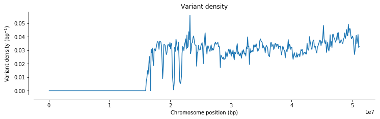
When working with large genotype arrays, scikit-allel has a GenotypeDaskArray class that is like the GenotypeArray class we met earlier but can handle data stored on-disk in HDF5 or Zarr files and compute over them without loading all data into memory.
gt = allel.GenotypeDaskArray(callset_h1k['22/calldata/GT'])
gt| 0 | 1 | 2 | 3 | 4 | ... | 2499 | 2500 | 2501 | 2502 | 2503 | ||
|---|---|---|---|---|---|---|---|---|---|---|---|---|
| 0 | 0/0 | 0/0 | 0/0 | 0/0 | 0/0 | ... | 0/0 | 0/0 | 0/0 | 0/0 | 0/0 | |
| 1 | 0/0 | 0/0 | 0/0 | 0/0 | 0/0 | ... | 0/0 | 0/0 | 0/0 | 0/0 | 0/0 | |
| 2 | 0/0 | 0/0 | 0/0 | 0/0 | 0/0 | ... | 0/0 | 0/0 | 0/0 | 0/0 | 0/0 | |
| ... | ... | |||||||||||
| 1103544 | 0/0 | 0/0 | 0/0 | 0/0 | 0/0 | ... | 0/0 | 0/0 | 0/0 | 0/0 | 0/0 | |
| 1103545 | 0/0 | 0/0 | 0/0 | 0/0 | 0/0 | ... | 0/0 | 0/0 | 0/0 | 0/0 | 0/0 | |
| 1103546 | 0/0 | 0/0 | 0/0 | 0/0 | 0/0 | ... | 0/0 | 0/0 | 0/0 | 0/0 | 0/0 | |
The main difference with the Dask-backed arrays is that you need to explicitly call compute() to run a computation, e.g.:
%%time
ac = gt.count_alleles(max_allele=8).compute()
CPU times: user 28 s, sys: 651 ms, total: 28.7 s
Wall time: 4.23 s
ac| 0 | 1 | 2 | 3 | 4 | 5 | 6 | 7 | 8 | ||
|---|---|---|---|---|---|---|---|---|---|---|
| 0 | 5007 | 1 | 0 | 0 | 0 | 0 | 0 | 0 | 0 | |
| 1 | 4976 | 32 | 0 | 0 | 0 | 0 | 0 | 0 | 0 | |
| 2 | 4970 | 38 | 0 | 0 | 0 | 0 | 0 | 0 | 0 | |
| ... | ... | |||||||||
| 1103544 | 4969 | 39 | 0 | 0 | 0 | 0 | 0 | 0 | 0 | |
| 1103545 | 5007 | 1 | 0 | 0 | 0 | 0 | 0 | 0 | 0 | |
| 1103546 | 4989 | 19 | 0 | 0 | 0 | 0 | 0 | 0 | 0 | |
Further reading
If you have any questions, please send an email to the scikit-allel mailing list. If you’re wondering where to go next, some of these articles may be of interest:
- Installing Python for data analysis
- A tour of scikit-allel
- Fast PCA
- Estimating FST
- Mendelian transmission
Further documentation about scikit-allel is available from the scikit-allel API docs.
Post-script: grouping by chromosome
In the worked example above, I had a VCF file with data from a single chromosome, and I used the “group” argument to extract the data into the Zarr store under a group named after the chromosome (“22”). This wasn’t strictly necessary for the worked example, but if I then wanted to extract data for other chromosomes, grouping the data by chromosome provides a convenient way to keep the data organised.
For example, if I also wanted to extract data for Chromosome 21, I would do the following:
vcf_path = 'data/ALL.chr21.phase3_shapeit2_mvncall_integrated_v5a.20130502.genotypes.vcf.gz'

allel.vcf_to_zarr(vcf_path, zarr_path, group='21',
                  fields='*', alt_number=8, log=sys.stdout,
                  compressor=numcodecs.Blosc(cname='zstd', clevel=1, shuffle=False))
[vcf_to_zarr] 65536 rows in 12.83s; chunk in 12.83s (5109 rows/s); 21�:15597733
[vcf_to_zarr] 131072 rows in 23.83s; chunk in 11.01s (5953 rows/s); 21�:17688253
[vcf_to_zarr] 196608 rows in 34.98s; chunk in 11.15s (5877 rows/s); 21�:19697865
[vcf_to_zarr] 262144 rows in 46.24s; chunk in 11.26s (5821 rows/s); 21�:21745371
[vcf_to_zarr] 327680 rows in 57.22s; chunk in 10.98s (5969 rows/s); 21�:23694335
[vcf_to_zarr] 393216 rows in 68.53s; chunk in 11.31s (5795 rows/s); 21�:25609367
[vcf_to_zarr] 458752 rows in 81.13s; chunk in 12.60s (5200 rows/s); 21�:27761870
[vcf_to_zarr] 524288 rows in 93.15s; chunk in 12.02s (5450 rows/s); 21�:29885097
[vcf_to_zarr] 589824 rows in 104.42s; chunk in 11.27s (5816 rows/s); 21�:32050808
[vcf_to_zarr] 655360 rows in 115.55s; chunk in 11.13s (5888 rows/s); 21�:34251524
[vcf_to_zarr] 720896 rows in 127.02s; chunk in 11.47s (5714 rows/s); 21�:36455104
[vcf_to_zarr] 786432 rows in 142.15s; chunk in 15.13s (4330 rows/s); 21�:38563725
[vcf_to_zarr] 851968 rows in 153.81s; chunk in 11.65s (5623 rows/s); 21�:40757642
[vcf_to_zarr] 917504 rows in 165.23s; chunk in 11.42s (5737 rows/s); 21�:42768192
[vcf_to_zarr] 983040 rows in 179.12s; chunk in 13.89s (4717 rows/s); 21�:44738104
[vcf_to_zarr] 1048576 rows in 191.46s; chunk in 12.34s (5309 rows/s); 21�:46520145
[vcf_to_zarr] 1105538 rows in 201.12s; chunk in 9.66s (5898 rows/s)
[vcf_to_zarr] all done (5488 rows/s)
Note that the vcf_path has changed because I’m extracting from a different VCF file, but I’m using the same zarr_path as before because the data will be grouped by chromosome within the Zarr store.
Here’s the new data hierarchy after extracting data for Chromosome 21:
callset_h1k.tree(expand=True)- /
- 21
- calldata
- GT (1105538, 2504, 2) int8
- samples (2504,) object
- variants
- AA (1105538,) object
- AC (1105538, 8) int32
- AF (1105538, 8) float32
- AFR_AF (1105538, 8) float32
- ALT (1105538, 8) object
- AMR_AF (1105538, 8) float32
- AN (1105538,) int32
- CHROM (1105538,) object
- CIEND (1105538, 2) int32
- CIPOS (1105538, 2) int32
- CS (1105538,) object
- DP (1105538,) int32
- EAS_AF (1105538, 8) float32
- END (1105538,) int32
- EUR_AF (1105538, 8) float32
- EX_TARGET (1105538,) bool
- FILTER_PASS (1105538,) bool
- ID (1105538,) object
- IMPRECISE (1105538,) bool
- MC (1105538,) object
- MEINFO (1105538, 4) object
- MEND (1105538,) int32
- MLEN (1105538,) int32
- MSTART (1105538,) int32
- MULTI_ALLELIC (1105538,) bool
- NS (1105538,) int32
- POS (1105538,) int32
- QUAL (1105538,) float32
- REF (1105538,) object
- SAS_AF (1105538, 8) float32
- SVLEN (1105538,) int32
- SVTYPE (1105538,) object
- TSD (1105538,) object
- VT (1105538,) object
- is_snp (1105538,) bool
- numalt (1105538,) int32
- svlen (1105538, 8) int32
- calldata
- 22
- calldata
- GT (1103547, 2504, 2) int8
- samples (2504,) object
- variants
- AA (1103547,) object
- AC (1103547, 8) int32
- AF (1103547, 8) float32
- AFR_AF (1103547, 8) float32
- ALT (1103547, 8) object
- AMR_AF (1103547, 8) float32
- AN (1103547,) int32
- CHROM (1103547,) object
- CIEND (1103547, 2) int32
- CIPOS (1103547, 2) int32
- CS (1103547,) object
- DP (1103547,) int32
- EAS_AF (1103547, 8) float32
- END (1103547,) int32
- EUR_AF (1103547, 8) float32
- EX_TARGET (1103547,) bool
- FILTER_PASS (1103547,) bool
- ID (1103547,) object
- IMPRECISE (1103547,) bool
- MC (1103547,) object
- MEINFO (1103547, 4) object
- MEND (1103547,) int32
- MLEN (1103547,) int32
- MSTART (1103547,) int32
- MULTI_ALLELIC (1103547,) bool
- NS (1103547,) int32
- POS (1103547,) int32
- QUAL (1103547,) float32
- REF (1103547,) object
- SAS_AF (1103547, 8) float32
- SVLEN (1103547,) int32
- SVTYPE (1103547,) object
- TSD (1103547,) object
- VT (1103547,) object
- is_snp (1103547,) bool
- numalt (1103547,) int32
- svlen (1103547, 8) int32
- calldata
- 21
If you want to save time, you could run the extraction for each chromosome in parallel, it is fine to write to a Zarr store from multiple processes.
The 1000 genomes project has built a separate VCF file for each chromosome, but you may have a single VCF file with data for multiple chromosomes. In this case you can still group the data by chromosome in the Zarr output, but you need to use the region argument when doing the extraction, and the VCF file needs to be tabix indexed. E.g.:
vcf_path = '/path/to/input.vcf.gz'  # tabix-indexed VCF with data for multiple chromosomes
zarr_path = '/path/to/output.zarr'
chromosomes = [str(i) for i in range(1, 23)]
for chrom in chromosomes:
    allel.vcf_to_zarr(vcf_path, zarr_path, group=chrom, region=chrom, ...)
Post-script: SNPEFF annotations
If you have a VCF with annotations from SNPEFF, you can post-process these to extract out data from within the ANN annotations. For example, here’s an example VCF with SNPEFF annotations:
with open('example_snpeff.vcf', mode='r') as f:
    print(f.read())
##fileformat=VCFv4.1
##INFO=<ID=AC,Number=A,Type=Integer,Description="Allele count in genotypes, for each ALT allele, in the same order as listed">
##FORMAT=<ID=GT,Number=1,Type=String,Description="Genotype">
##SnpEffVersion="4.1b (build 2015-02-13), by Pablo Cingolani"
##SnpEffCmd="SnpEff agam4.2 -noStats -lof - "
##INFO=<ID=ANN,Number=.,Type=String,Description="Functional annotations: 'Allele | Annotation | Annotation_Impact | Gene_Name | Gene_ID | Feature_Type | Feature_ID | Transcript_BioType | Rank | HGVS.c | HGVS.p | cDNA.pos / cDNA.length | CDS.pos / CDS.length | AA.pos / AA.length | Distance | ERRORS / WARNINGS / INFO' ">
#CHROM POS ID REF ALT QUAL FILTER INFO
2L 103 . C T 53.36 . AC=4;ANN=T|intergenic_region|MODIFIER|AGAP004677|AGAP004677|intergenic_region|AGAP004677||||||||3000|
2L 192 . G A 181.16 . AC=8;
2L 13513722 . A T,G 284.06 PASS AC=1;ANN=T|missense_variant|MODERATE|AGAP005273|AGAP005273|transcript|AGAP005273-RA|VectorBase|1/4|n.17A>T|p.Asp6Val|17/4788|17/4788|6/1596||,G|synonymous_variant|LOW|AGAP005273|AGAP005273|transcript|AGAP005273-RA|VectorBase|1/4|n.17A>G|p.Asp6Asp|12/4768|12/4768|4/1592||
The main thing to note is that the values of the ANN field contain multiple sub-fields. E.g., in the first variant, the ANN value is “T|intergenic_region|MODIFIER|AGAP004677|AGAP004677|intergenic_region|AGAP004677||||||||3000|”. The sub-fields are delimited by the pipe character (“|”). The first sub-field gives the allele to which the effect annotation applies (“T”); the second sub-field gives the effect annotation (“intergenic_region”); etc.
By default, scikit-allel parses the ANN field like any other string field, e.g.:
callset = allel.read_vcf('example_snpeff.vcf', fields='ANN')
ann = callset['variants/ANN']
ann
array([ 'T|intergenic_region|MODIFIER|AGAP004677|AGAP004677|intergenic_region|AGAP004677||||||||3000|',
'',
'T|missense_variant|MODERATE|AGAP005273|AGAP005273|transcript|AGAP005273-RA|VectorBase|1/4|n.17A>T|p.Asp6Val|17/4788|17/4788|6/1596||'], dtype=object)
However, like this the data aren’t much use. If you want to access the sub-fields, scikit-allel provides a transformers parameter, which can be used like this:
callset = allel.read_vcf('example_snpeff.vcf', fields='ANN', transformers=allel.ANNTransformer())
list(callset)
['variants/ANN_AA_length',
'variants/ANN_AA_pos',
'variants/ANN_Allele',
'variants/ANN_Annotation',
'variants/ANN_Annotation_Impact',
'variants/ANN_CDS_length',
'variants/ANN_CDS_pos',
'variants/ANN_Distance',
'variants/ANN_Feature_ID',
'variants/ANN_Feature_Type',
'variants/ANN_Gene_ID',
'variants/ANN_Gene_Name',
'variants/ANN_HGVS_c',
'variants/ANN_HGVS_p',
'variants/ANN_Rank',
'variants/ANN_Transcript_BioType',
'variants/ANN_cDNA_length',
'variants/ANN_cDNA_pos']
Note that even though I only requested the “ANN” field, the resulting callset has a number of fields, each of which represents a sub-field from the ANN annotation. E.g.:
callset['variants/ANN_Allele']array(['T', '', 'T'], dtype=object)
callset['variants/ANN_Annotation']array(['intergenic_region', '', 'missense_variant'], dtype=object)
You can also use the transformers parameter with other functions, e.g.:
df = allel.vcf_to_dataframe('example_snpeff.vcf', fields='ANN', transformers=allel.ANNTransformer())
df| ANN_Allele | ANN_Annotation | ANN_Annotation_Impact | ANN_Gene_Name | ANN_Gene_ID | ANN_Feature_Type | ANN_Feature_ID | ANN_Transcript_BioType | ANN_Rank | ANN_HGVS_c | ANN_HGVS_p | ANN_cDNA_pos | ANN_cDNA_length | ANN_CDS_pos | ANN_CDS_length | ANN_AA_pos | ANN_AA_length | ANN_Distance | |
|---|---|---|---|---|---|---|---|---|---|---|---|---|---|---|---|---|---|---|
| 0 | T | intergenic_region | MODIFIER | AGAP004677 | AGAP004677 | intergenic_region | AGAP004677 | -1 | -1 | -1 | -1 | -1 | -1 | -1 | 3000 | |||
| 1 | -1 | -1 | -1 | -1 | -1 | -1 | -1 | -1 | ||||||||||
| 2 | T | missense_variant | MODERATE | AGAP005273 | AGAP005273 | transcript | AGAP005273-RA | VectorBase | 1 | 17A>T | Asp6Val | 17 | 4788 | 17 | 4788 | 6 | 1596 | -1 |
One thing to watch out for, some variants can have multiple SNPEFF annotations, i.e., there can be multiple values for the ANN annotation. This can happen if a variant has multiple alleles, or if a variant is within a gene that has multiple transcripts, or if a variant is within two overlapping genes (e.g., on opposite strands, or one gene within an intron of another), or if genes are closely spaced and so you get an upstream or downstream annotation for one gene and another annotation for the gene the variant is in, or some combination of any or all of these.
E.g., in the example above, the third variant has two alternate alleles, and therefore has two ANN values, and by default only the first value has been parsed. You can increase the number of values via the numbers parameter as usual, e.g.:
callset = allel.read_vcf('example_snpeff.vcf', fields='ANN', numbers={'ANN': 2},
transformers=allel.ANNTransformer())callset['variants/ANN_Allele']array([['T', ''],
['', ''],
['T', 'G']], dtype=object)
callset['variants/ANN_Annotation']array([['intergenic_region', ''],
['', ''],
['missense_variant', 'synonymous_variant']], dtype=object)
Dealing with multiple SNPEFF annotations can be tricky. FWIW my suggestion is, when generating the SNPEFF annotations, use the option to only call annotations against the canonical (longest) transcript for each gene, and disable upstream and downstream annotations. This will at least reduce some of the complexity, although you’ll still need to handle multiallelic variants and the odd case of overlapping genes.
Post-script: changes from vcfnp
The new functions available in scikit-allel supercede a package I previously wrote for extracting data from VCF files called vcfnp. I rewrote this functionality from the ground up and ported the functionality to scikit-allel for two main reasons. Firstly, vcfnp was slow and so you needed a cluster to parse big VCF files, which is obviously a pain. The new functions in scikit-allel should be up to ~40 times faster. Secondly, the vcfnp API was somewhat complicated, requiring three separate steps to get data from VCF into an HDF5 file or Zarr store. The new functions in scikit-allel hopefully simplify this process, enabling data to be extracted from VCF and loaded into any of a variety of storage containers via a single function call.
If you previously used vcfnp here are a few notes on some of the things that have changed.
- No need for separate function calls to extract data from variants and calldata fields, both can be extracted via a single call to
read_vcf()or any of thevcf_to_...()functions described above. - Data can be extracted from VCF and loaded into HDF5 with a single function call to
vcf_to_hdf5(); i.e., no need to first extract parts of the data out to .npy files then load into HDF5. - No need to use a cluster or do any parallelisation, it should be possible to run
vcf_to_hdf5()orvcf_to_zarr()on a whole VCF on a half-decent desktop or laptop computer, although big VCF files might take a couple of hours and require a reasonably large hard disk. - The default NumPy data type for string fields has changed to use ‘object’ dtype, which means that strings of any length will be stored automatically (i.e., no need to configure separate dtypes for each string field) and there will be no truncation of long strings.
- Previously in
vcfnpthe genotype calls were extracted into a special field called ‘genotype’ separate from the ‘GT’ calldata field if requested. Inscikit-allelthe default behaviour is to parse the ‘GT’ field as a 3-dimensional integer array and return simply as ‘calldata/GT’. If you really want to process the ‘GT’ field as a string then you can override this by setting the type for ‘calldata/GT’ to ‘S3’ or ‘object’. - The “arity” argument in
vcfnpis instead called “numbers” in scikit-allel, to match better with the terminology used in VCF meta-information headers. - Genotype ploidy is now specified via the “numbers” argument, there is no special “ploidy” argument.